Feed Forward Neural Network (FFNN) adalah arsitektur artificial neural network di mana informasi mengalir satu arah dari input ke output tanpa loops .
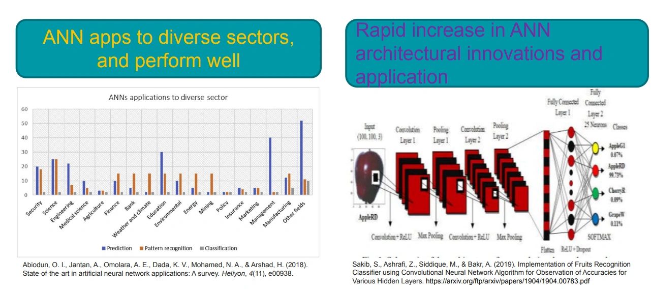
ANN berhasil diterapkan di berbagai sektor: image recognition, NLP, time-series ANN terbukti berhasil di berbagai sektor. ANN cocok untuk masalah dengan karakteristik:
Instances direpresentasikan oleh banyak attribute-value pairs
Target function bisa discrete-valued , real-valued , atau vektor
Training examples boleh mengandung noise/errors
Waktu training yang lama dapat diterima
Evaluasi cepat dari fungsi target yang dipelajari diperlukan
Kemampuan manusia memahami hasil pembelajaran tidak penting
Perceptron (termasuk Adaline): satu unit/neuron, fungsi estimasi.
Artificial Neural Network : banyak computational units yang menjadi intelligent hanya melalui interaksi satu sama lain , terinspirasi dari otak, dan terdiri dari komposisi banyak fungsi berbeda.
Single layer Neural Network dengan update rule:
w ← w + η ( y − y ^ ) ⋅ x w \leftarrow w + \eta (y - \hat{y}) \cdot x w ← w + η ( y − y ^ ) ⋅ x
Error menggunakan Squared Error loss function . Disebut juga Widrow-Hoff rule atau LMS rule , yang merupakan bridge antara Perceptron dan FFNN.
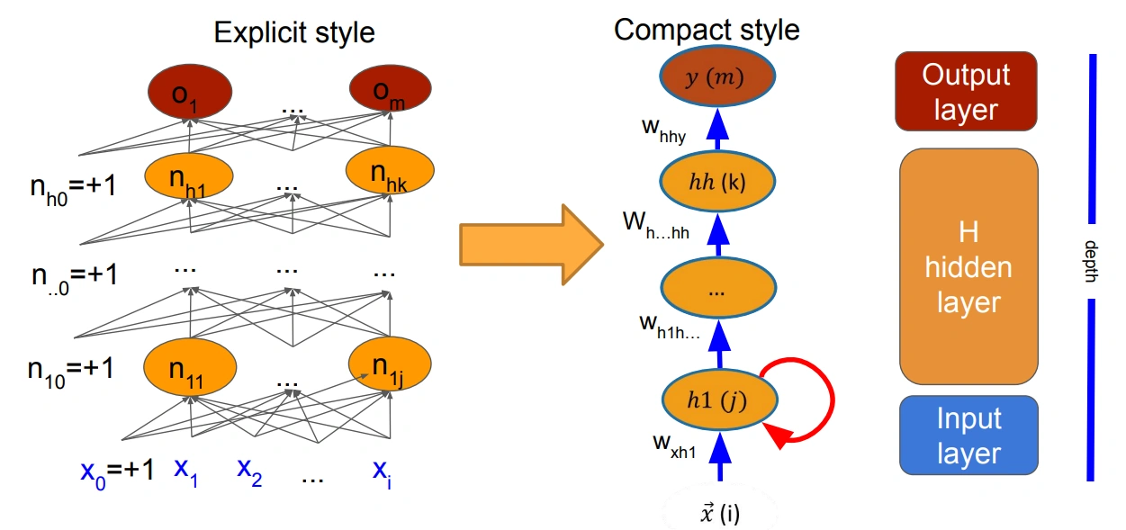
Arsitektur ANN: explicit style (diagram lengkap) dan compact style (notasi matriks) Arsitektur FFNN terdiri dari:
Setiap layer terhubung sepenuhnya (fully connected ) ke layer berikutnya.
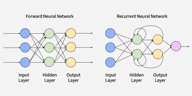
FFNN: directed acyclic graph; RNN: ada loops untuk sequence processing Arsitektur Deskripsi Feed Forward Neural Network (FFNN) Koneksi hanya satu arah, membentuk directed acyclic graph (DAG). Tidak ada loops . Multi Layer Perceptron (MLP) FFNN yang fully connected dengan fungsi aktivasi non-linear . Recurrent Neural Network (RNN) Memiliki loops berupa output intermediate /final di-feed back sebagai input. Dibahas lebih lanjut di bagian RNN.
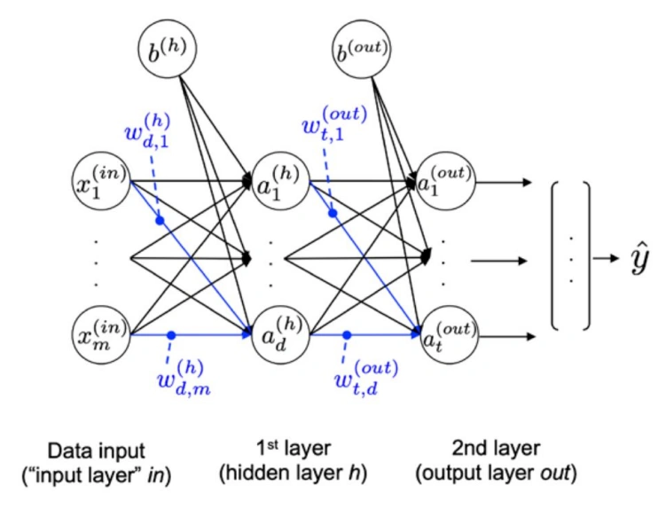
2-layer MLP: input layer tidak dihitung, hidden + output = 2 layer
Dalam beberapa konteks, input juga dianggap sebagai layer. Namun pada konvensi umum, layer dihitung dari hidden dan output sehingga Adaline (single hidden unit) adalah single-layer network , dan MLP standar dengan satu hidden layer adalah two-layer network .
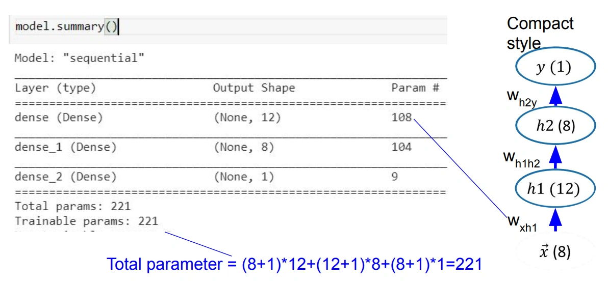
Jumlah parameter: setiap koneksi + bias adalah parameter yang dapat dilatih Total parameter = jumlah bobot + jumlah bias.
Param per layer = ( input units + 1 ) × output units \text{Param per layer} = (\text{input units} + 1) \times \text{output units} Param per layer = ( input units + 1 ) × output units
Contoh: Input (8), HL1 (12), HL2 (8), Output (1):
Total = ( 8 + 1 ) × 12 + ( 12 + 1 ) × 8 + ( 8 + 1 ) × 1 = 108 + 104 + 9 = 221 \text{Total} = (8+1) \times 12 + (12+1) \times 8 + (8+1) \times 1 = 108 + 104 + 9 = \mathbf{221} Total = ( 8 + 1 ) × 12 + ( 12 + 1 ) × 8 + ( 8 + 1 ) × 1 = 108 + 104 + 9 = 221
Implementasi Keras:
from keras.models import Sequential from keras.layers import Dense
model = Sequential() model.add(Dense( 12 , input_dim = 8 , activation = ' relu ' )) model.add(Dense( 8 , activation = ' relu ' )) model.add(Dense( 1 , activation = ' sigmoid ' ))
model.compile( loss = ' binary_crossentropy ' , optimizer = ' adam ' , metrics = [ ' accuracy ' ]) model.fit(X, y, epochs = 150 , batch_size = 10 )
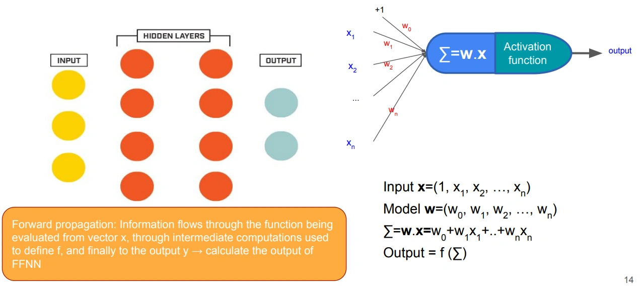
Forward propagation: input mengalir melalui network dari kiri ke kanan Informasi mengalir melalui network dari input ke output untuk menghitung prediksi.
Untuk input vector x \mathbf{x} x W x h W_{xh} W x h c \mathbf{c} c W h y W_{hy} W h y b \mathbf{b} b
f ( x ; W x h , c , W h y , b ) = f 2 ( W h y T ⋅ f 1 ( W x h T ⋅ x + c ) + b ) f(\mathbf{x};\, W_{xh}, \mathbf{c}, W_{hy}, \mathbf{b}) = f_2\!\left(W_{hy}^T \cdot f_1\!\left(W_{xh}^T \cdot \mathbf{x} + \mathbf{c}\right) + \mathbf{b}\right) f ( x ; W x h , c , W h y , b ) = f 2 ( W h y T ⋅ f 1 ( W x h T ⋅ x + c ) + b )
Jika bias dimasukkan ke dalam matriks bobot:
f ( x ; W x h , W h y ) = f 2 ( W h y T ⋅ f 1 ( W x h T ⋅ x ) ) f(\mathbf{x};\, W_{xh}, W_{hy}) = f_2\!\left(W_{hy}^T \cdot f_1\!\left(W_{xh}^T \cdot \mathbf{x}\right)\right) f ( x ; W x h , W h y ) = f 2 ( W h y T ⋅ f 1 ( W x h T ⋅ x ) )
Untuk input mini-batch X X X
f ( X ; W x h , c , W h y , b ) = f 2 ( f 1 ( X ⋅ W x h + c ) ⋅ W h y + b ) f(X;\, W_{xh}, \mathbf{c}, W_{hy}, \mathbf{b}) = f_2\!\left(f_1(X \cdot W_{xh} + \mathbf{c}) \cdot W_{hy} + \mathbf{b}\right) f ( X ; W x h , c , W h y , b ) = f 2 ( f 1 ( X ⋅ W x h + c ) ⋅ W h y + b )
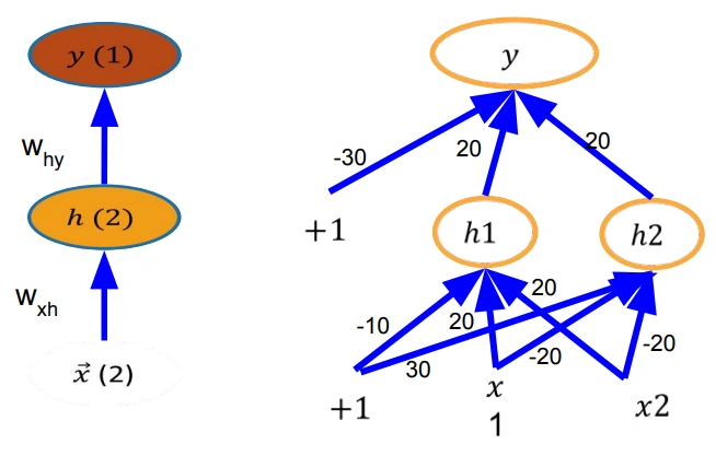
XOR dengan sigmoid: 2 hidden units mampu merepresentasikan XOR yang tidak linearly separable x 1 x_1 x 1 x 2 x_2 x 2 y y y 0 0 0 0 1 1 1 0 1 1 1 0
h 1 = σ ( − 10 + 20 x 1 + 20 x 2 ) , h 2 = σ ( 30 − 20 x 1 − 20 x 2 ) h_1 = \sigma(-10 + 20x_1 + 20x_2), \quad h_2 = \sigma(30 - 20x_1 - 20x_2) h 1 = σ ( − 10 + 20 x 1 + 20 x 2 ) , h 2 = σ ( 30 − 20 x 1 − 20 x 2 )
y = σ ( − 30 + 20 h 1 + 20 h 2 ) y = \sigma(-30 + 20h_1 + 20h_2) y = σ ( − 30 + 20 h 1 + 20 h 2 )
h 1 = ReLU ( 0 + x 1 + x 2 ) , h 2 = ReLU ( − 1 + x 1 + x 2 ) h_1 = \text{ReLU}(0 + x_1 + x_2), \quad h_2 = \text{ReLU}(-1 + x_1 + x_2) h 1 = ReLU ( 0 + x 1 + x 2 ) , h 2 = ReLU ( − 1 + x 1 + x 2 )
y = 0 + h 1 − 2 h 2 y = 0 + h_1 - 2h_2 y = 0 + h 1 − 2 h 2
Verifikasi untuk ( x 1 = 1 , x 2 = 1 ) (x_1=1, x_2=1) ( x 1 = 1 , x 2 = 1 )
h 1 = ReLU ( 2 ) = 2 h_1 = \text{ReLU}(2) = 2 h 1 = ReLU ( 2 ) = 2 h 2 = ReLU ( 1 ) = 1 h_2 = \text{ReLU}(1) = 1 h 2 = ReLU ( 1 ) = 1 y = 2 − 2 ( 1 ) = 0 y = 2 - 2(1) = 0 y = 2 − 2 ( 1 ) = 0
Fungsi Formula Range Turunan Linear f ( z ) = z f(z) = z f ( z ) = z ( − ∞ , + ∞ ) (-\infty, +\infty) ( − ∞ , + ∞ ) f ′ ( z ) = 1 f'(z) = 1 f ′ ( z ) = 1 Sigmoid f ( z ) = 1 1 + e − z f(z) = \frac{1}{1 + e^{-z}} f ( z ) = 1 + e − z 1 ( 0 , 1 ) (0, 1) ( 0 , 1 ) f ′ ( z ) = f ( z ) ( 1 − f ( z ) ) f'(z) = f(z)(1 - f(z)) f ′ ( z ) = f ( z ) ( 1 − f ( z )) ReLU f ( z ) = max ( 0 , z ) f(z) = \max(0, z) f ( z ) = max ( 0 , z ) [ 0 , + ∞ ) [0, +\infty) [ 0 , + ∞ ) f ′ ( z ) = 1 f'(z) = 1 f ′ ( z ) = 1 z > 0 z > 0 z > 0 0 0 0 z ≤ 0 z \leq 0 z ≤ 0
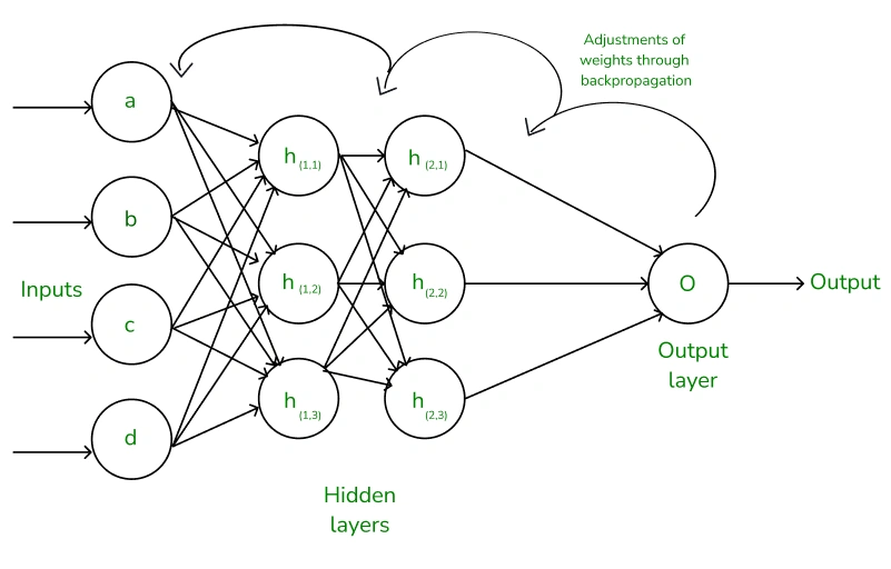
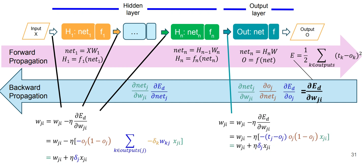
Learning procedure: forward prop → compute error → backward prop → update weights Backpropagation adalah algoritma untuk melatih FFNN dengan cara menghitung gradient error terhadap setiap bobot menggunakan chain rule .
Forward propagation : hitung output
y y y untuk input
x x x Backward propagation : hitung
error term δ \delta δ untuk setiap neuron
Update setiap bobot berdasarkan error term
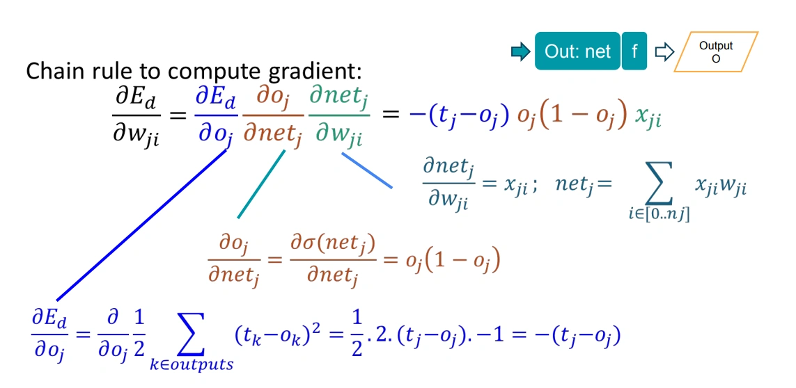
Backprop MLP: error mengalir mundur dari output layer ke hidden layers Gradient untuk output unit weights: δ_o = -(t-o)·f'(net) Untuk output unit dengan loss function E E E
δ o = ∂ E ∂ net o = − ( t − o ) ⋅ f ′ ( net o ) \delta_o = \frac{\partial E}{\partial \text{net}_o} = -(t - o) \cdot f'(\text{net}_o) δ o = ∂ net o ∂ E = − ( t − o ) ⋅ f ′ ( net o )
Jika menggunakan aktivasi sigmoid:
δ o = − ( t − o ) ⋅ o ( 1 − o ) \delta_o = -(t - o) \cdot o(1 - o) δ o = − ( t − o ) ⋅ o ( 1 − o )
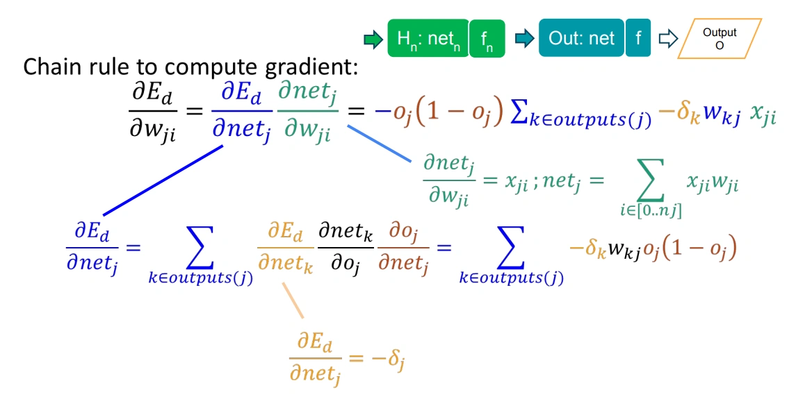
Gradient untuk hidden unit weights: δ_h = f'(net_h) · Σ(w_hk · δ_k) Untuk hidden unit h h h
δ h = f ′ ( net h ) ⋅ ∑ k ∈ outputs w h k ⋅ δ k \delta_h = f'(\text{net}_h) \cdot \sum_{k \in \text{outputs}} w_{hk} \cdot \delta_k δ h = f ′ ( net h ) ⋅ ∑ k ∈ outputs w hk ⋅ δ k
Jika hidden unit menggunakan sigmoid:
δ h = o h ( 1 − o h ) ⋅ ∑ k ∈ outputs w h k ⋅ δ k \delta_h = o_h(1 - o_h) \cdot \sum_{k \in \text{outputs}} w_{hk} \cdot \delta_k δ h = o h ( 1 − o h ) ⋅ ∑ k ∈ outputs w hk ⋅ δ k
w i j new = w i j old − η ⋅ ∂ E ∂ w i j = w i j old − η ⋅ δ j ⋅ x i w_{ij}^{\text{new}} = w_{ij}^{\text{old}} - \eta \cdot \frac{\partial E}{\partial w_{ij}} = w_{ij}^{\text{old}} - \eta \cdot \delta_j \cdot x_i w ij new = w ij old − η ⋅ ∂ w ij ∂ E = w ij old − η ⋅ δ j ⋅ x i
Karena δ \delta δ − ( t − o ) -(t-o) − ( t − o )
w i j new = w i j old + η ⋅ ( t − o ) ⋅ f ′ ( net ) ⋅ x i w_{ij}^{\text{new}} = w_{ij}^{\text{old}} + \eta \cdot (t - o) \cdot f'(\text{net}) \cdot x_i w ij new = w ij old + η ⋅ ( t − o ) ⋅ f ′ ( net ) ⋅ x i
Dua konvensi backpropagation:
Konvensi kalkulus :
δ = ∂ E ∂ net = − ( t − o ) ⋅ f ′ \delta = \frac{\partial E}{\partial \text{net}} = -(t-o) \cdot f' δ = ∂ net ∂ E = − ( t − o ) ⋅ f ′ , update:
w = w − η ⋅ δ ⋅ x w = w - \eta \cdot \delta \cdot x w = w − η ⋅ δ ⋅ x (
subtraktif ).
δ \delta δ bernilai
positif ketika output melebihi target.
Konvensi Mitchell (pseudocode di bawah):
δ = ( t − o ) ⋅ f ′ \delta = (t-o) \cdot f' δ = ( t − o ) ⋅ f ′ , update:
w = w + η ⋅ δ ⋅ x w = w + \eta \cdot \delta \cdot x w = w + η ⋅ δ ⋅ x (
aditif ).
δ \delta δ bernilai
negatif ketika output melebihi target.
Tanda negatif "berpindah" antara definisi δ \delta δ identik .
Petunjuk membaca soal ujian:
Jika soal mendefinisikan
δ = ∂ E ∂ net \delta = \frac{\partial E}{\partial \text{net}} δ = ∂ net ∂ E atau
− ( t − o ) -(t-o) − ( t − o ) → konvensi kalkulus.
Jika soal menulis
δ = ( t − o ) ⋅ f ′ \delta = (t-o) \cdot f' δ = ( t − o ) ⋅ f ′ atau
w = w + η ⋅ δ ⋅ x w = w + \eta \cdot \delta \cdot x w = w + η ⋅ δ ⋅ x → konvensi Mitchell.
Initialize all weights to small random values
Until termination condition is met:
    For each training example <x, t>:
        // Forward pass
        Compute output o for each unit

        // Backward pass (output units)
        For each output unit k:
            δ_k = o_k(1 - o_k)(t_k - o_k)

        // Backward pass (hidden units, from output back to first hidden)
        For each hidden unit h:
            δ_h = o_h(1 - o_h) * Σ(w_hk * δ_k)

        // Weight update
        For each weight w_ij:
            w_ij = w_ij + η * δ_j * x_i
Termination conditions:
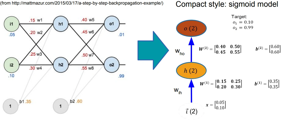
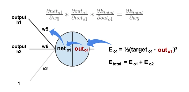
Backprop contoh: 2 input → 2 hidden (sigmoid) → 2 output (sigmoid), η=0.5 Arsitektur: 2 input, 2 hidden (sigmoid), 2 output (sigmoid), η = 0.5 \eta = 0.5 η = 0.5
Setup:
i 1 = 0.05 i_1 = 0.05 i 1 = 0.05 ,
i 2 = 0.10 i_2 = 0.10 i 2 = 0.10 w 1 = 0.15 w_1 = 0.15 w 1 = 0.15 ,
w 2 = 0.20 w_2 = 0.20 w 2 = 0.20 ,
w 3 = 0.25 w_3 = 0.25 w 3 = 0.25 ,
w 4 = 0.30 w_4 = 0.30 w 4 = 0.30 (input → hidden)
w 5 = 0.40 w_5 = 0.40 w 5 = 0.40 ,
w 6 = 0.45 w_6 = 0.45 w 6 = 0.45 ,
w 7 = 0.50 w_7 = 0.50 w 7 = 0.50 ,
w 8 = 0.55 w_8 = 0.55 w 8 = 0.55 (hidden → output)
b 1 = 0.35 b_1 = 0.35 b 1 = 0.35 (bias hidden),
b 2 = 0.60 b_2 = 0.60 b 2 = 0.60 (bias output)
Target:
t 1 = 0.01 t_1 = 0.01 t 1 = 0.01 ,
t 2 = 0.99 t_2 = 0.99 t 2 = 0.99 Hidden layer:
net h 1 = w 1 i 1 + w 2 i 2 + b 1 = 0.15 ( 0.05 ) + 0.20 ( 0.10 ) + 0.35 = 0.3775 \text{net}_{h_1} = w_1 i_1 + w_2 i_2 + b_1 = 0.15(0.05) + 0.20(0.10) + 0.35 = 0.3775 net h 1 = w 1 i 1 + w 2 i 2 + b 1 = 0.15 ( 0.05 ) + 0.20 ( 0.10 ) + 0.35 = 0.3775 o h 1 = σ ( 0.3775 ) = 0.5933 o_{h_1} = \sigma(0.3775) = 0.5933 o h 1 = σ ( 0.3775 ) = 0.5933
net h 2 = w 3 i 1 + w 4 i 2 + b 1 = 0.25 ( 0.05 ) + 0.30 ( 0.10 ) + 0.35 = 0.3925 \text{net}_{h_2} = w_3 i_1 + w_4 i_2 + b_1 = 0.25(0.05) + 0.30(0.10) + 0.35 = 0.3925 net h 2 = w 3 i 1 + w 4 i 2 + b 1 = 0.25 ( 0.05 ) + 0.30 ( 0.10 ) + 0.35 = 0.3925 o h 2 = σ ( 0.3925 ) = 0.5969 o_{h_2} = \sigma(0.3925) = 0.5969 o h 2 = σ ( 0.3925 ) = 0.5969
Output layer:
net o 1 = w 5 o h 1 + w 6 o h 2 + b 2 = 0.40 ( 0.5933 ) + 0.45 ( 0.5969 ) + 0.60 = 1.1059 \text{net}_{o_1} = w_5 o_{h_1} + w_6 o_{h_2} + b_2 = 0.40(0.5933) + 0.45(0.5969) + 0.60 = 1.1059 net o 1 = w 5 o h 1 + w 6 o h 2 + b 2 = 0.40 ( 0.5933 ) + 0.45 ( 0.5969 ) + 0.60 = 1.1059 o 1 = σ ( 1.1059 ) = 0.7514 o_1 = \sigma(1.1059) = 0.7514 o 1 = σ ( 1.1059 ) = 0.7514
net o 2 = w 7 o h 1 + w 8 o h 2 + b 2 = 0.50 ( 0.5933 ) + 0.55 ( 0.5969 ) + 0.60 = 1.2250 \text{net}_{o_2} = w_7 o_{h_1} + w_8 o_{h_2} + b_2 = 0.50(0.5933) + 0.55(0.5969) + 0.60 = 1.2250 net o 2 = w 7 o h 1 + w 8 o h 2 + b 2 = 0.50 ( 0.5933 ) + 0.55 ( 0.5969 ) + 0.60 = 1.2250 o 2 = σ ( 1.2250 ) = 0.7729 o_2 = \sigma(1.2250) = 0.7729 o 2 = σ ( 1.2250 ) = 0.7729
Total Error:
E = 1 2 ( t 1 − o 1 ) 2 + 1 2 ( t 2 − o 2 ) 2 = 1 2 ( 0.01 − 0.7514 ) 2 + 1 2 ( 0.99 − 0.7729 ) 2 = 0.2748 + 0.0236 = 0.2984 E = \frac{1}{2}(t_1 - o_1)^2 + \frac{1}{2}(t_2 - o_2)^2 = \frac{1}{2}(0.01 - 0.7514)^2 + \frac{1}{2}(0.99 - 0.7729)^2 = 0.2748 + 0.0236 = \mathbf{0.2984} E = 2 1 ( t 1 − o 1 ) 2 + 2 1 ( t 2 − o 2 ) 2 = 2 1 ( 0.01 − 0.7514 ) 2 + 2 1 ( 0.99 − 0.7729 ) 2 = 0.2748 + 0.0236 = 0.2984
Backprop example backward pass: gradient mengalir dari output ke hidden ke input Error term output units (konvensi Mitchell: δ = ( t − o ) ⋅ f ′ \delta = (t-o) \cdot f' δ = ( t − o ) ⋅ f ′
δ o 1 = o 1 ( 1 − o 1 ) ( t 1 − o 1 ) = 0.7514 × 0.2486 × ( − 0.7414 ) = − 0.1385 \delta_{o_1} = o_1(1 - o_1)(t_1 - o_1) = 0.7514 \times 0.2486 \times (-0.7414) = \mathbf{-0.1385} δ o 1 = o 1 ( 1 − o 1 ) ( t 1 − o 1 ) = 0.7514 × 0.2486 × ( − 0.7414 ) = − 0.1385
δ o 2 = o 2 ( 1 − o 2 ) ( t 2 − o 2 ) = 0.7729 × 0.2271 × 0.2171 = 0.0381 \delta_{o_2} = o_2(1 - o_2)(t_2 - o_2) = 0.7729 \times 0.2271 \times 0.2171 = \mathbf{0.0381} δ o 2 = o 2 ( 1 − o 2 ) ( t 2 − o 2 ) = 0.7729 × 0.2271 × 0.2171 = 0.0381
Error term hidden units:
δ h 1 = o h 1 ( 1 − o h 1 ) ⋅ ( w 5 δ o 1 + w 7 δ o 2 ) = 0.5933 × 0.4067 × ( 0.40 × ( − 0.1385 ) + 0.50 × 0.0381 ) = − 0.00876 \delta_{h_1} = o_{h_1}(1 - o_{h_1}) \cdot (w_5 \delta_{o_1} + w_7 \delta_{o_2}) = 0.5933 \times 0.4067 \times (0.40 \times (-0.1385) + 0.50 \times 0.0381) = \mathbf{-0.00876} δ h 1 = o h 1 ( 1 − o h 1 ) ⋅ ( w 5 δ o 1 + w 7 δ o 2 ) = 0.5933 × 0.4067 × ( 0.40 × ( − 0.1385 ) + 0.50 × 0.0381 ) = − 0.00876
δ h 2 = o h 2 ( 1 − o h 2 ) ⋅ ( w 6 δ o 1 + w 8 δ o 2 ) = 0.5969 × 0.4031 × ( 0.45 × ( − 0.1385 ) + 0.55 × 0.0381 ) = − 0.00994 \delta_{h_2} = o_{h_2}(1 - o_{h_2}) \cdot (w_6 \delta_{o_1} + w_8 \delta_{o_2}) = 0.5969 \times 0.4031 \times (0.45 \times (-0.1385) + 0.55 \times 0.0381) = \mathbf{-0.00994} δ h 2 = o h 2 ( 1 − o h 2 ) ⋅ ( w 6 δ o 1 + w 8 δ o 2 ) = 0.5969 × 0.4031 × ( 0.45 × ( − 0.1385 ) + 0.55 × 0.0381 ) = − 0.00994
Output layer weights (w = w + η ⋅ δ j ⋅ x i w = w + \eta \cdot \delta_j \cdot x_i w = w + η ⋅ δ j ⋅ x i
Bobot Update Nilai Baru w 5 w_5 w 5 0.40 + 0.5 × ( − 0.1385 ) × 0.5933 0.40 + 0.5 \times (-0.1385) \times 0.5933 0.40 + 0.5 × ( − 0.1385 ) × 0.5933 0.3589 0.3589 0.3589 w 6 w_6 w 6 0.45 + 0.5 × ( − 0.1385 ) × 0.5969 0.45 + 0.5 \times (-0.1385) \times 0.5969 0.45 + 0.5 × ( − 0.1385 ) × 0.5969 0.4087 0.4087 0.4087 w 7 w_7 w 7 0.50 + 0.5 × 0.0381 × 0.5933 0.50 + 0.5 \times 0.0381 \times 0.5933 0.50 + 0.5 × 0.0381 × 0.5933 0.5113 0.5113 0.5113 w 8 w_8 w 8 0.55 + 0.5 × 0.0381 × 0.5969 0.55 + 0.5 \times 0.0381 \times 0.5969 0.55 + 0.5 × 0.0381 × 0.5969 0.5614 0.5614 0.5614
Hidden layer weights:
Bobot Update Nilai Baru w 1 w_1 w 1 0.15 + 0.5 × ( − 0.00876 ) × 0.05 0.15 + 0.5 \times (-0.00876) \times 0.05 0.15 + 0.5 × ( − 0.00876 ) × 0.05 0.14978 0.14978 0.14978 w 2 w_2 w 2 0.20 + 0.5 × ( − 0.00876 ) × 0.10 0.20 + 0.5 \times (-0.00876) \times 0.10 0.20 + 0.5 × ( − 0.00876 ) × 0.10 0.19956 0.19956 0.19956 w 3 w_3 w 3 0.25 + 0.5 × ( − 0.00994 ) × 0.05 0.25 + 0.5 \times (-0.00994) \times 0.05 0.25 + 0.5 × ( − 0.00994 ) × 0.05 0.24975 0.24975 0.24975 w 4 w_4 w 4 0.30 + 0.5 × ( − 0.00994 ) × 0.10 0.30 + 0.5 \times (-0.00994) \times 0.10 0.30 + 0.5 × ( − 0.00994 ) × 0.10 0.29950 0.29950 0.29950
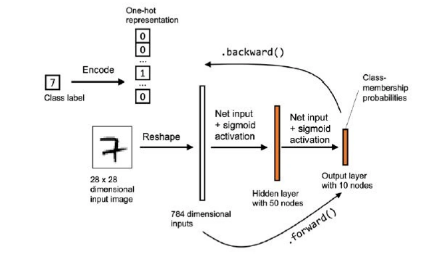
NN untuk digit tulisan tangan: input 784 → hidden layers → output 10 kelas Klasifikasi digit tulisan tangan (MNIST 28×28 = 784 piksel) menggunakan FFNN:
Input (784) → Hidden 1 (128, ReLU) → Hidden 2 (64, ReLU) → Output (10, Softmax)
Aspek Keterangan Arsitektur Input → Hidden Layer(s) → Output Forward Propagation Hitung output dari input ke output Backpropagation Hitung error terms dari output ke input (chain rule) Weight Update (Mitchell) w = w + η ⋅ δ ⋅ x w = w + \eta \cdot \delta \cdot x w = w + η ⋅ δ ⋅ x Weight Update (Kalkulus) w = w − η ⋅ δ ⋅ x w = w - \eta \cdot \delta \cdot x w = w − η ⋅ δ ⋅ x Aktivasi Sigmoid, ReLU, Linear Loss Function Squared Error: E = 1 2 ( t − o ) 2 E = \frac{1}{2}(t-o)^2 E = 2 1 ( t − o ) 2 Vanishing Gradient Sigmoid di jaringan dalam → gradient mengecil → gunakan ReLU